Cooling coil in an AHU: capacity and dehumidification calculation

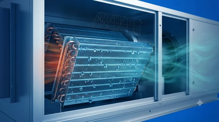
The cooling coil in an air handling unit (AHU) cools the supply air below its dew point — condensing out the excess moisture and draining it away as condensate. The total cooling capacity is the sum of the sensible and latent heat: $\Phi_c = \dot{m} \cdot (h_1 - h_2)$, where $h_1$ and $h_2$ are the air enthalpies before and after the coil.

The principle of cooling with dehumidification

The air enters the coil at temperature $t_1$ and relative humidity $\varphi_1$. The coil cools it through the dew point ($t_d$) to the outlet temperature $t_2$:

1. Sensible cooling — a drop in temperature with no change in humidity, until the air reaches its dew point
2. Latent cooling (dehumidification) — below the dew point the water vapor condenses, and the humidity ratio $x$ falls
3. Outlet state — the air leaves the coil saturated ($\varphi_2 \approx 95\text{–}100\%$) or is subsequently reheated to the required temperature

The principle of cooling without dehumidification

If the outlet temperature $t_2$ stays above the dew-point temperature, no condensation occurs — the air is merely cooled.

1. Sensible cooling — a drop in temperature with no change in humidity, until the air reaches its dew point
2. Outlet state — the air leaves the coil more saturated than at the inlet

Calculating the cooling capacity

Total cooling capacity

$$\Phi_c = \dot{m} \cdot (h_1 - h_2) \quad \text{[kW]}$$

where $\dot{m}$ is the air mass flow rate [kg/s].

The sensible component

$$\Phi_s = \dot{m} \cdot c_{pa} \cdot (t_1 - t_2) \approx \dot{m} \cdot 1.006 \cdot (t_1 - t_2) \quad \text{[kW]}$$

The latent component (dehumidification)

$$\Phi_{lat} = \dot{m} \cdot r_0 \cdot (x_1 - x_2) \approx \dot{m} \cdot 2501 \cdot (x_1 - x_2) \quad \text{[kW]}$$

where $r_0 = 2501\ \text{kJ/kg}$ is the latent heat of water at 0 °C.

Condensate flow

$$q_{\text{cond}} = \dot{m} \cdot (x_1 - x_2)\ \text{[kg/s]} = \dot{m} \cdot (x_1 - x_2) \cdot 3600\ \text{[l/h]}$$

A worked example

Given: an AHU, flow rate 3000 m³/h, coil inlet: $t_1$ = 32 °C, $φ_1$ = 55%, outlet: $t_2$ = 14 °C, $φ_2$ = 95%.

Psychrometric values:

• Air density: $\rho \approx 1.145\ \text{kg/m}^3$ → $\dot{m} = \frac{3000}{3600} \cdot 1.145 = \mathbf{0.955}\ \textbf{kg/s}$
• $h_1$ (32 °C, φ 55%): $\approx \mathbf{74.6}\ \textbf{kJ/kg}$
• $h_2$ (14 °C, φ 95%): $\approx \mathbf{38.1}\ \textbf{kJ/kg}$
• $x_1 \approx 16.6\ \text{g/kg}$, $x_2 \approx 9.5\ \text{g/kg}$

Results:

• Total capacity: $\Phi_c = 0.955 \cdot (74.6 - 38.1) = \mathbf{34.9}\ \textbf{kW}$
• Sensible capacity: $\Phi_s = 0.955 \cdot 1.006 \cdot (32 - 14) = \mathbf{17.3}\ \textbf{kW}$
• Latent capacity: $\Phi_{lat} = 0.955 \cdot 2501 \cdot \dfrac{16.6 - 9.5}{1000} = \mathbf{17.0}\ \textbf{kW}$
• Condensate: $0.955 \cdot \dfrac{7.1}{1000} \cdot 3600 = \mathbf{24.4}\ \textbf{l/h}$

Sensible heat ratio (SHR)

The SHR (Sensible Heat Ratio) gives the share of the total cooling capacity that is sensible cooling:

$$\text{SHR} = \frac{\Phi_s}{\Phi_c} = \frac{17.3}{34.9} = \mathbf{0.50}$$

Typical values:

• Offices: SHR = 0.75–0.85 (low internal latent-heat production)
• Restaurants, pools: SHR = 0.45–0.65
• Tropical climate: SHR = 0.50–0.65

The temperature after the coil (bypass factor)

A real coil never cools all the air exactly to the surface temperature of the exchanger. The bypass factor (BF) = the fraction of air that passes through the coil without contact:

$$t_2 = t_{\text{ADP}} + \text{BF} \cdot (t_1 - t_{\text{ADP}})$$

where $t_{\text{ADP}}$ is the apparatus dew point temperature — the surface temperature of the exchanger.

The BF for a finned exchanger is typically 0.05–0.15. On the Mollier diagram, the outlet-air state lies on the line connecting the state $t_1$, $\varphi_1$ with the saturation curve — the distance corresponds to the BF.

Cooling on the Mollier diagram

On the h-x diagram:

1. Plot the inlet air state (point 1)
2. Draw a line to the left toward the saturation curve — point 2’ is the ideal outlet (BF = 0)
3. The actual outlet (point 2) lies on the segment 1–2’ at a distance BF from the saturation curve

You can also work the construction through by hand — a blank sheet to print draws the saturation curve at 0.5 mm, so it is easy to aim at with a ruler. PsychroView performs this calculation automatically once you enter the inlet state and the outlet temperature or enthalpy.

Frequently asked questions

How do I find the cooling capacity I need? The cooling capacity is set by the room’s heat gains (sun, people, luminaires, equipment) plus the heat brought in by ventilation. For a standard office, reckon on 60–100 W/m² of total cooling capacity.

Why is the coil outlet saturated air? The coil cools the air below its dew point — moisture condenses and the air approaches saturation. Downstream of the coil the air is typically φ = 90–100% and relatively cold (12–16 °C), which is why a reheater is usually placed after the coil.

What is a chilled-water coil and a DX coil? Chilled-water coil (CW) — cold water (typically +6/+12 °C) from a central cooling source (a chiller) flows through the fins. DX coil (direct expansion) — refrigerant evaporates in the fins directly from a compressor unit.